The Evenden-Brunner-Inversion. Only a small program in my map projection colletion but an importing closing of a an painful gap in map projection theory.
The common map projection formulas transformes the spheric Earth surface coodinates longitude λ and latitude φ into the map coordinates x and y (direct transformation). But often inverse formulas are needed to transform a map-x,y-pair into λ and φ.
The Winkel Tripel of Oswald Winkel 1921 (most cites from Wagner 1949/S. 224 as 1913) is one of the most popular map projection. But it is not invertable in a closed analytical form. And it is not a running implementation known.
Cengizhan Ipbüker/I. Öztug Bildirici have publicated in 2002 (see below) a Winkel-Tripel-Inversion method in theory. G. I. Evenden gives in Issue 2008 Libroj.4 manual a Aïtoff inversion solution. Jakob Brunner, Luzern has me sent a Winkel Inversion Excel solution by means of Newton-Raphson-Iteration.
With best regards to Jakob Brunner, Luzern.
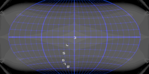
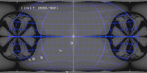
Test run #1 - First implementation test
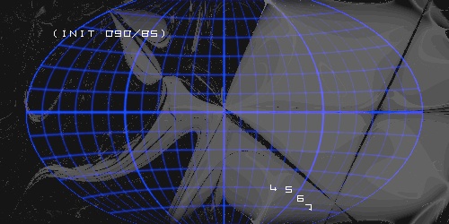
Brunners original initial point arc 1/1 (alias 57/57 degree, near Perm, Russia). One iteration gives a linear approimation ...
2 iterations - quadratic approximation ...
3 iterations, cubic solution ...
5 iterations -
10 iterations -
Okay - it runs and may become a Winkel Tripel. But it is still some to do ...
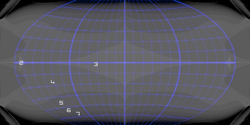
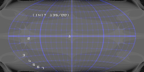
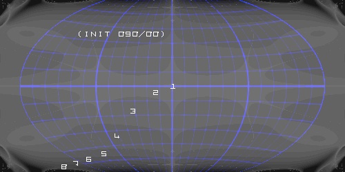
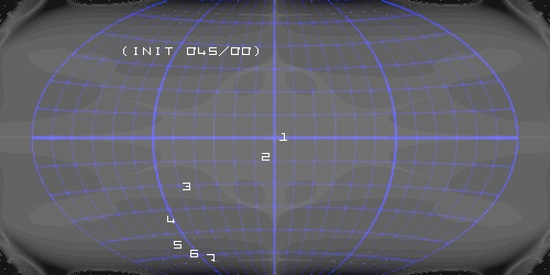
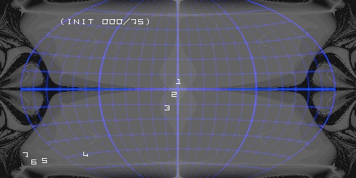
Test run #2 - New convergence raw
We take initial point 1 degree E 1 degree N. Linear ...
Quadratic ...
Cubic ...
But higher appoximations, here 5 gives a bad divergence gap on outer equatorial areas.
10 cycles:
20 cycles.
OK, it is a Winkel Tripel. But note the visible gap at outer (far east and west) equator. That's a problem. Also a (more academic) problem is the assymetry caused by the 1 E 1 N located inital point - near the image centre but outside of any symmetry axis.
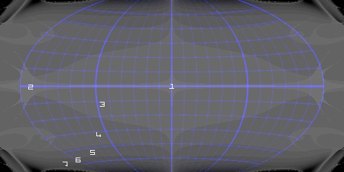
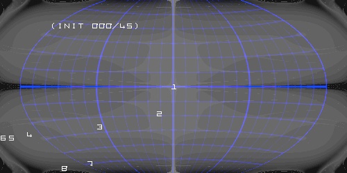
Test run #3 - Iteration step analysis ...
More deeper analyzing. We change algorithm and indicator. We take a epsilon value as precision target and count and write the needed steps as grey value in each pixel. Black means bad convergence (>15 iteration steps), lighter and more lighter grey a rising better convergence. The numbers are the numbers of iteration steps to reach the epsilon accuracy ...
What is the influence of epsilon? Epsilon=0.000000001 („convergence class e-09“) is Brunners original value.
Initial point in that row is is E 180 N 0. It gives good solutions near the equator but near the poles are needed 20 ... 30 iterations.
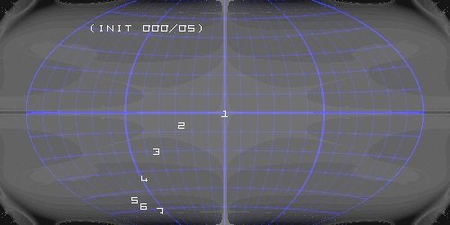
A lower epsilon=0.0000001 („convergence class e-07“) gives a larger convergence area ...
Here epsilon=0.00001 ...
Greather epsilons cause less iteration steps and a faster computation but a lower precision. The epsilon of 0.00000001 ist optimal. It also is the by Brunner recommended value.
Test run #4 - Some interesting images
Now a further search for initial points. As temporary work epsilon we use 0.0001 (ce-05) ...
Full central initialisation at 0 E 0 N shows a bad solution. We see the „latitude-45-degree-limitation“:

Initialization point 45 E 45 N (near brunners 57/57 „natural arc“ perm point) gives convergence images similar above in test run #1 ...
At a coffee break: Start point 85 E 90 N gives a very smart design ...
Test run #5 - Systematical search along equator
Now a systematic search for an intial point along the equator. We know from test run #3: 180 E 0 N gives a good convergence - except near the poles.

We shift the initial point along the equator inside the map centre, 135 E 0 N ...
90 E 0 N ...
45 E 0 N ...
No better convergence near the poles.
0 E 0 N - thats the image wirth the „latitude-45-degree-limitation“ ...

Better solutions but still suboptimal.
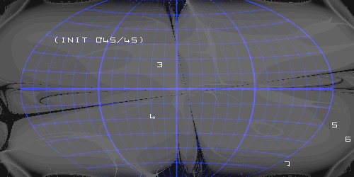
Test run #6 - Systematical search along greenwich meridian
Now a search for the initial point along the central meridian.
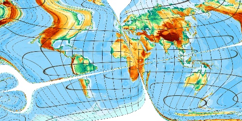
North pole initialization gives large (black) fractal gaps arround the equator in far east and far west ...
0 E 75 N ... decreasing latitude gives smaller gaps ...
0 E 45 N ... better, but still bad convergence on outer equator ...
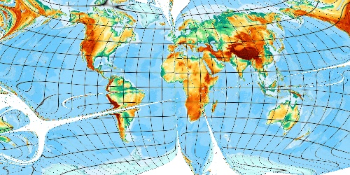
But I'm angry. At 0 E 0 N will come the „latitude-45-degree-limitation“. We take 5 N 0 E ...
... okay ... and now 0 E 1 N ...
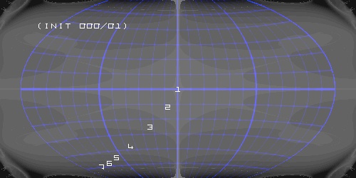
We risk further decreasing very near to the equator, 0 E 0.0625 degree N:
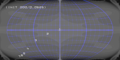
Very good! We note 0 E 0.062570 N as best result.
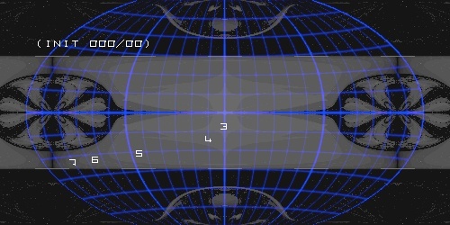
At end of this raw initial point 0 N 0 E (equator) gives the known image with the „latitude-45-degree-limitation“:
0 E 0.0625 is found as the best initial point!
Okay, it runs. And now the Release runs ...
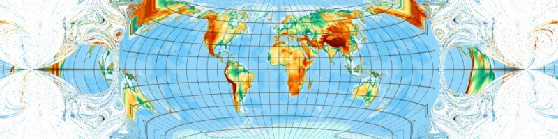
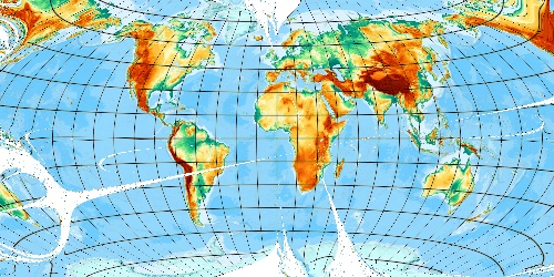
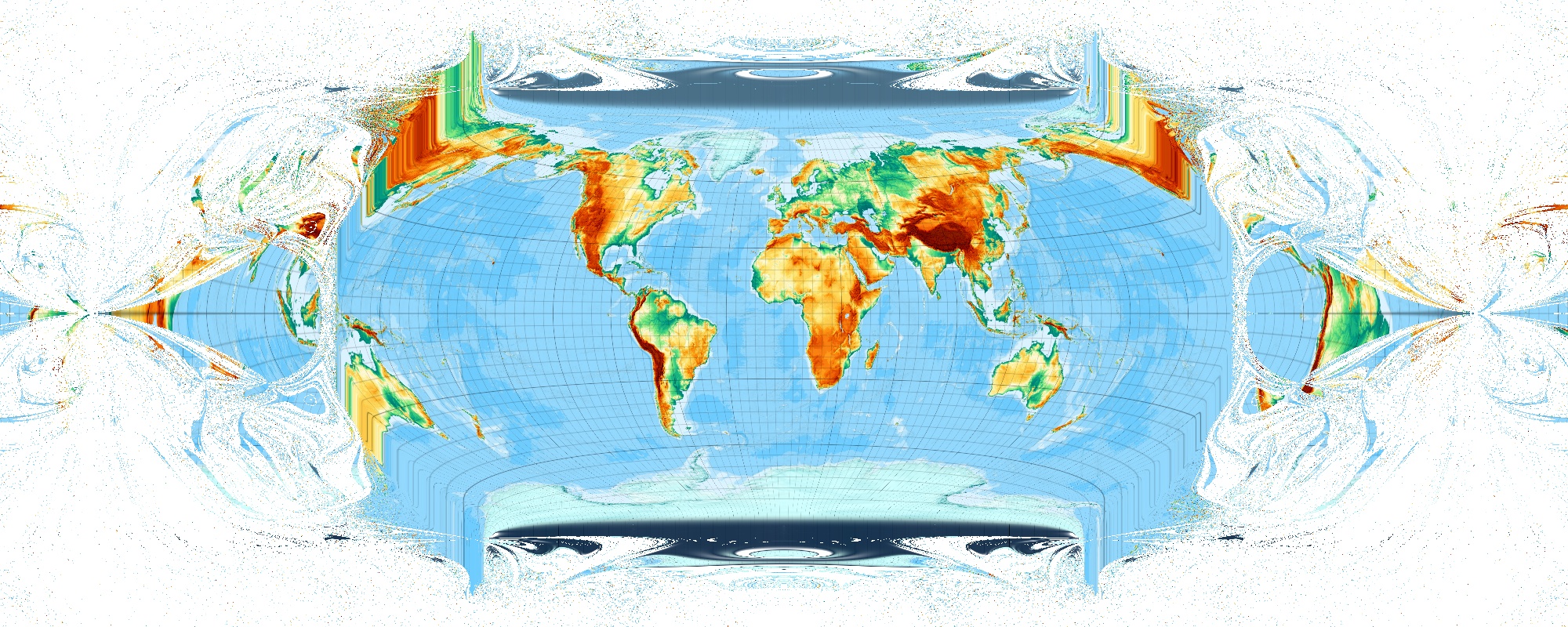
Test run #7 - A very large codomain map
We have found good convergence conditions: initial point latitude 0.0625 degree, longitude 0 degree, epsilon 1E-09. To demonstrate it, we compute a „very large codomain map“, half default scale, 1:600.000.000 ...
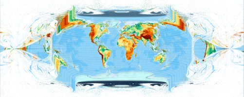
It shows: Latitudes > 90 and longitudes > 180 also often gives a practicable results. It is possible to compute pixel outside pole and date line. OK, there is no need for outside pole pixels, but to compute outside date line pixel - that can make sense.
Large codomain map 1:400.000.000 (944 kByte)
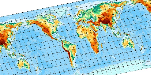
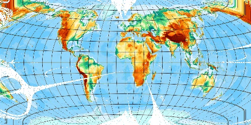
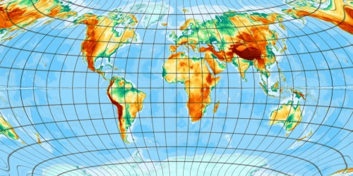
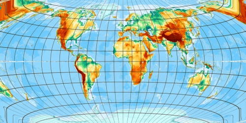
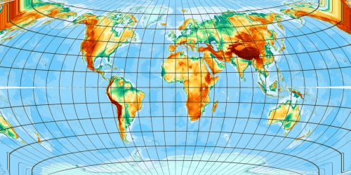
The Release run
It runs and now - the release map ...
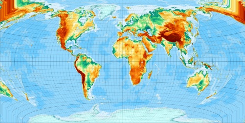
Large image 1:400.000.000 (188 kByte)
Large image 1:200.000.000 (931 kByte)
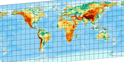
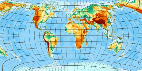
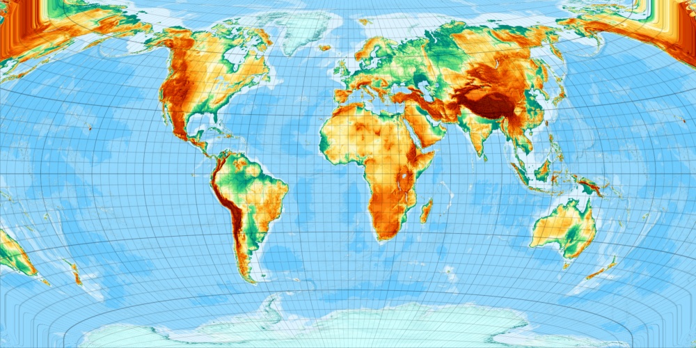
Here a compasision with direct generation:
It is the same map. But note: a function and its inverse change their codomain and image. The inverse runs all over the map and the Evenden-Brunner-Interation also gives a solution outside the date line.
Literature:
Cengizhan Ipbüker, I. Öztug Bildirici, 2002: A General Algorithm fot the Inverse Transformation of Map Projections Using Jacobian Matrices Proceedings of the Third International Symposium Mathematical & Computational Applications September 4-6, 2002. Konya, Turkey, pp. 175-182 [Insbesondere mit einer Winkel Tripel Inversion.] http://atlas.selcuk.edu.tr/paperdb/papers/130.pdf
Böhm, R.: Variationen von Weltkartennetzen der Wagner-Hammer-Aïtoff-Entwurfsfamilie. Kartographische Nachrichten 56. Jg., Nr. 1., p. 8-16. - Kirschbaum: Bonn 2006.
Brunner, Jakob, Luzern 1020: Mail Correspondence.
Canters, F., 2002: Small-scale Map Projection Design (p. 185). London: Taylor & Francis 2002.
Evenden, G.I., 2008: Issue 2008 Libproj.4 manual
Grafarend, Erik, Krumm, Friedrich W., 2006: Map Projections. Berlin: Springer 2006.
Wagner, K.: Kartographische Netzentwürfe. Leipzig: Bibliographisches Instutut 1949, S. 224.
Winkler, O.: Neue Gradnetzkombinationen. Gotha: Perthes, Petermanns Geographische Nachrichten (Dezember) 1921. Band 67, S. 248-252
Deutscher Originaltext, ohne Bilder ·
Translation into englisch by M. Scherer, Karlsruhe, with Pictures
Wird meist als „Winkel 1913“ zitiert, was möglicherweise auf Wagner (1949, S. 224) zurückgeht. Ich bedanke mich herzlich bei Tobias Jung für diese Mitteilung.